Boundary Layer

Figure 1 – Lovely Heidelberg, departing point of boundary layer

The interaction of air with a body generates a space region where the air conditions are different from the freestream conditions. That region is named boundary layer. In basic air data applications we’re dealing with the need to make accurate freestream conditions measurements, so we’re really concerned about boundary layers.

Boundary layers have been studied since the very beginning of aerodynamics. In 1904 a twenty-nine years old Ludwig Prandtl lay down the grounds for modern aerodynamics with a short boundary layer presentation in Heidelberg[1].

So let’s visualize a boundary layer over a flat plate, refer to figure 2.
We have depicted a laminar air flow, velocity vectors highlight a marked velocity profile. The air flowing near the wall is slower than the air far from the wall, so the local velocity $u(y)$ is correlated to the distance from wall $y$ .

The boundary layer is defined as the region where the local velocity values $u(y)$ are less or equal than the 99% value (or other reference value) of the freestream value $u_infty$ .

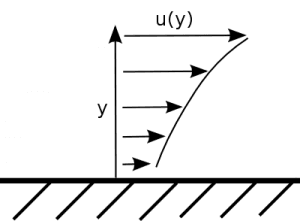
Figure 2 – Laminar flow boundary layer velocity profile

The speed at wall is zero. Air is viscous so to move one air layer with respect to other is necessary to apply a force.

Let’s consider the flow (Couette flow) between two parallel flat plates of area $A$ at a distance $y$ , one fixed to ground and the other free to move.
The force $F$ needed to maintain the speed $u$ of the moving plate is $F=\mu A\frac{\displaystyle u}{\displaystyle y}$ . The newly introduced parameter $\mu$ is the air dynamic viscosity, SI unit of measurement is $Pas$ . It is evident that is needed energy to maintain a boundary layer of given characteristics between the two plates.

In general boundary layers are affected by the fluid relative speed, fluid properties and body geometry; see the video 1, that visualize an example of laminar and turbulent flow.
Simplest way to visualize a boundary layer is to run a CFD simulation of a tube, you find a tutorial here.

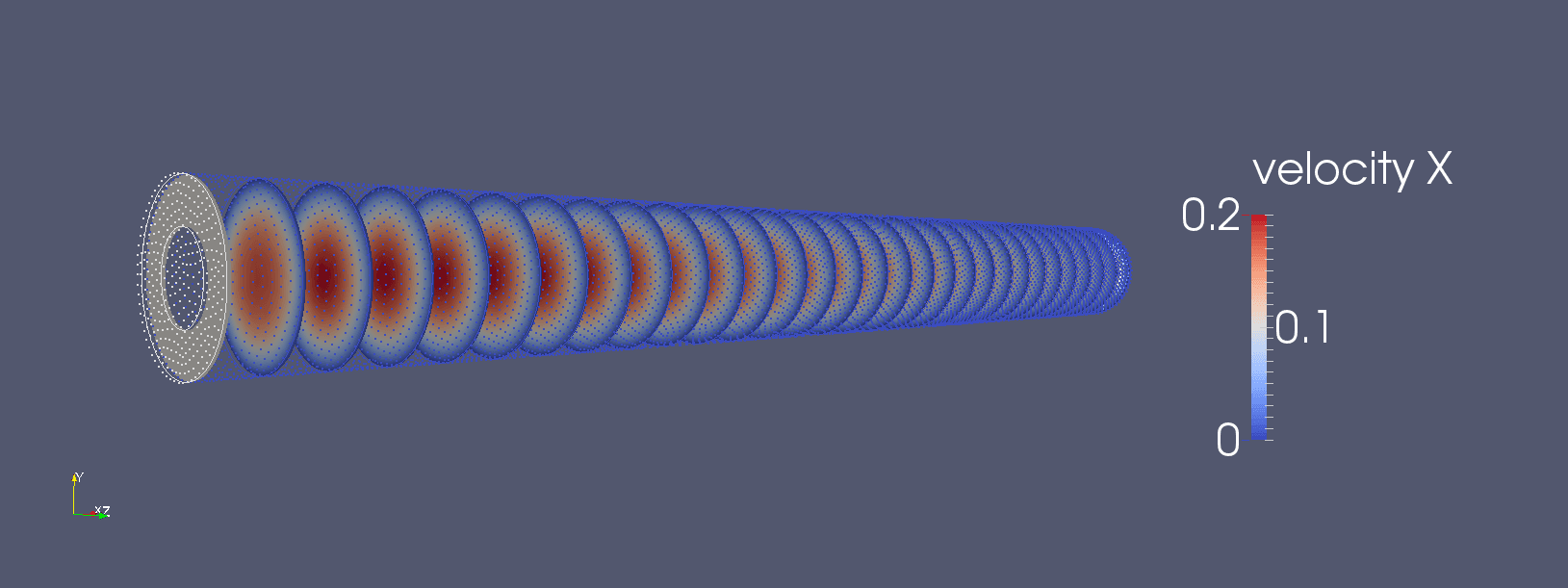
Figure 3 – Boundary layer velocity profiles in CFD pipe

From the figure 3 it is evident that the boundary layer is present and changes its shape along the pipe, the boundary changes with position so the flow is say to be developing along the longitudinal axis. Let’s pretend we want to calculate the flowrate across the pipe measuring the speed of the fluid at a single point inside the pipe.

Flowrate is the integral over time of the velocity across a fixed section multiplied by the fluid density Eq 12.2. To reconstruct the velocity values on the whole integration section with a single measurement we need to know the analytical expression of velocity profile, in many cases, that information, can be gathered from precedent research works.

It is evident that if we use the only measured velocity value as mean speed, neglecting the boundary layer, then we get a wrong flowrate measurement value.

Let’s change scenario, let’s pretend that we want to know the true airspeed of a racing car, refer to figure 4.

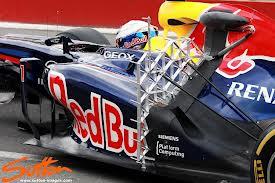
Figure 4 – Pitot rake on a race car

The issue here is that airspeed measured within the boundary layer is lower than the freestream airspeed. How far should protrude our pitot from the car body to work properly? Look this page for an analytical introductory approach.

At a glance to deal with a boundary layer we need to know:

Boundary layer thickness;
Boundary layer velocity distribution and flow status; turbulent, laminar or transition?
Flow development patterns, where the flow will change from laminar to turbulent?

In our typical application we’re dealing with a flying platform, where unfortunately the boundary layer characteristics change with the aircraft attitude and airspeed. For example the wing downwash affects all the posterior parts of the fuselage. Magnitude and pattern of airflow are dependent on the angle of attack.

In the real world it is non trivial to find a position that is not affected by the aircraft attitude. To push the measurement performances further, CFD, wind gallery study and inflight calibration are needed.

Until now we addressed our attention to the air velocity field, the same definition of boundary layer can be used to define a temperature boundary layer; both boundary layers impact on basic air data measurements.

Flow type and Reynolds Number

The Reynolds number can be used to predict a flow pattern. The onset of very fascinating flow patterns, for example vortex streets (Tutorial here) can be detected with the use of Reynolds numbers.

Depending on many factors, like fluid type and plate roughness the transition to turbulent flow will happen at a different Reynolds number. A plausible interval of values is:

$1^5 < Re < 3^6$

The larger the x-coordinate of the section we examine is, the wider the corresponding boundary layer will be. Given a section at a coordinate $x$ , we observe that the thickness of the corresponding boundary layer decreases as the free stream speed increases.

The Reynolds number is the ratio between inertial and viscous forces. A low Reynolds number indicates that inertial forces are overwhelmed by viscous forces. Conversely a high Reynolds number indicates that inertial forces are driving the flow.

We can distinguish three principal flow patterns: laminar, transitional and turbulent.

We have a laminar flow when the fluid flows in parallel layers, each layer having little interaction with the adjacent layer. In a laminar flow it is possible to distinguish parallel flowing streamlines. An extreme example of laminar flow is shown on the Video 2.

This flow has a very low Reynolds number, well below unity. As the flow is strongly laminar the operator can rewind the system to a state visually identical to the original state

Turbulent flow is characterized by an apparent randomness, circulation, eddies and high Reynolds number.

A transitional flow is somewhat in between the two previous cases: some parts of the fluid can have a laminar behavior and some others a turbulent-like behavior.

Determining the Reynolds number for each pattern in the transtional flow is not trivial, but fortunately for many notable cases there is an approximate math model. In the Video Various types of flow a complete transition between laminar and turbulent flow into a pipe is shown.

In the relevant literature, one of the most well-studied boundary layer patterns is the one formed by a flow over a flat plate. Under some assumptions, the boundary layer expression can be analytically found, for example there is the Blasius solution.

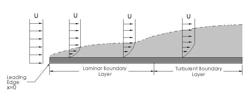
Figure 5 – Boundary layer over a flat plate

Have a look at Figure 5. One important thing to observe is that the boundary layer is developing along the plate $x$ coordinate, on the horizontal direction of the image. The Reynolds number expression is $Re=\rho Ux/\mu$ and $x=0$ corresponds to the leading edge of the plate or the beginning of the boundary layer itself. Initially, the flow is laminar and as $x$ increases the Reynolds number increases as well.

At some point, the boundary layer transforms into a transitional pattern and finally ends with a turbulent configuration. If one is able to increase $x$ at will, the flow will become turbulent sooner or later.

We can distinguish three principal flow patterns: laminar, transitional and turbulent.

This flow has a very low Reynolds number, well below unity. As the flow is strongly laminar the operator can rewind the system to a state visually identical to the original state

Turbulent flow is characterized by an apparent randomness, circulation, eddies and high Reynolds number.

A transitional flow is somewhat in between the two previous cases: some parts of the fluid can have a laminar behavior and some others a turbulent-like behavior.

We can observe the relationship between freestream speed and boundary layer thickness on the Video Spatially developing turbulence.

In the Video Spatially developing turbulence, the transition to turbulent pattern is triggered by an aerodynamic obstacle. Pressure gradients can cause transitions of boundary layers. Pressure gradients are likely to occur on external air temperature probes inside the diffuser section. You can see the geometry of a Kiel probe here.

In the general case, boundary layer shape is time and position dependent and thus no overall closed form solution is available.

References

[1]

J. D.Anderson, “Ludwig Prandtl’s Boundary Layer,” Physics Today, 2005 [Online]. Available: https://www.aps.org/units/dfd/resources/upload/prandtl_vol58no12p42_48.pdf>

Flow type and Reynolds Number

Further reading

References